Coding theory, interactive quizzes & live code

This page shows an example on how to combine the introduction of a certain coding implementation with interactive questions. Compared to the previous template, the learning objective is to learn a new skill in programming using the live coding feature whereas before programming was used to illustrate a theoretic concept unrelated to coding (for example statistics).

Example unconstrained optimization

In this chapter, we’ll cover how to apply scipy.optimize.minimize to unconstrained optimization problems. As a reminder, unconstrained optimization considers:

(4)\[\mathop {\min }\limits_x f\left( x \right)\]

with \(x\) the design variable of length \(n\) and \(f\) the objective function.

Method

In this course, we’re making use of the function scipy.optimize.minimize. The documentation of this function is available here: https://docs.scipy.org/doc/scipy/reference/generated/scipy.optimize.minimize.html. In this course we’ll cover only the relevant parts.

For unconstrained optimization we need to run at least scipy.optimize.minimize(fun, x0, ...) with:

• fun, the objective function \(f(x)\) to be minimized. fun is a callable. The scipy.optmize.minimize function takes care of defining and inputing our design variable \(x\).

• x0, the initial guess for our design variable \(x\). It needs to be a ndarray with length \(n\)

The function scipy.optimize.minimize outputs an object scipy.optimize.OptimizeResult. with:

• scipy.optimize.OptimizeResult.x the optimized solution of the design variable x. It is a ndarray with length \(n\)

• scipy.optimize.OptimizeResult.success, a indication whether or not the optimizer was executed succesfully. It is a bool, indicating True or False

• scipy.optimize.OptimizeResult.message, a message describing the cause of termination of the optimizatino algorithm. It is a str.

• scipy.optimize.OptimizeResult.fun, the values of the optimized objective function \(f\). It is a int or float

• scipy.optimize.OptimizeResult.nit, the number of iteration performed by the optimizer. It is a int

Example 1

Problem

It is desired to determine the number of bathymetry maps \(n\) of a local area that should be produced to maximize the profit of a company. The total cost of production and distribution is €\(75\) per unit \(n\). The revenues are proportional to the number of units multiplied by its price: \(Revenues = n \cdot Price \)

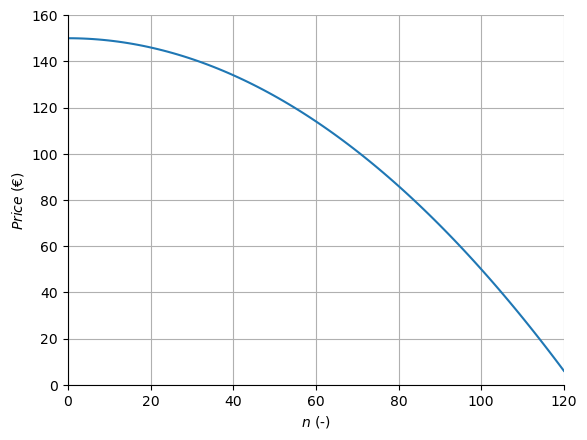
The demand depends on the price (\(Price = 150 - 0.01n^2\)), as shown in the graph:

The profit can be estimated as the revenues minus the total costs.

Model

The function for the profit can be found by combining the relations in the problem statement. However, this is the profit which should be maximized. To turn this into a minimization problem, the profit can be multiplied with \(-1\). The final model of this problem results in:

(5)\[\mathop {\min }\limits_n \left(75n - \left( 150 - 0.01n^2 \right) n \right)\]

Method

This model is described using scipy.optimize.minimize.

Importing libraries

import scipy as sp 
import numpy as np
import matplotlib.pylab as plt

Defining the variables

There are very few variables in this problem. In fact, the only variable we have to specify is the initial guess for the optimization algorithm. The objective function will be treated later. The length of \(n\) doesn’t have to be specified.

n0 = 20

Defining the objective function

In the objective function, the formula given in the model description can be inserted. Or, each individual step can be calculated on a seperate line. Again, note that the profit is multiplied with \(-1\) to maximize the profit in the minimization formulation. This results in:

def negprofit(n):
    price = 150 - 0.01 * n**2
    revenues = price * n
    totalcost = 75 * n
    profit = revenues - totalcost
    return -profit

Solving the problem

Now, the problem can be solved. The result is stored in the variables result which is printed.

result = sp.optimize.minimize(negprofit,n0)
print(result)

  message: Optimization terminated successfully.
  success: True
   status: 0
      fun: -2499.9999999998727
        x: [ 5.000e+01]
      nit: 8
      jac: [ 0.000e+00]
 hess_inv: [[ 3.503e-01]]
     nfev: 22
     njev: 11

Postprocessing

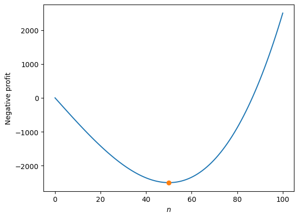
As this case is only one-dimensional and the potential range of values is limited, we can easily check this answer by an exhaustive search, evaluating all possible values for \(n\). The plot below shows the \(\text{negative profit}\) for \(0<n<100\). It shows a clear minimum which coincides with the minimum found by scipy.optimize.minimize

n_range = np.linspace(0,100,100)
negprofit_result = negprofit(n_range)
plt.plot(n_range,negprofit_result)
plt.plot(result.x,result.fun,'o');
plt.xlabel('$n$')
plt.ylabel('Negative profit');

Exercise

Adapt the code to answer the following questions.